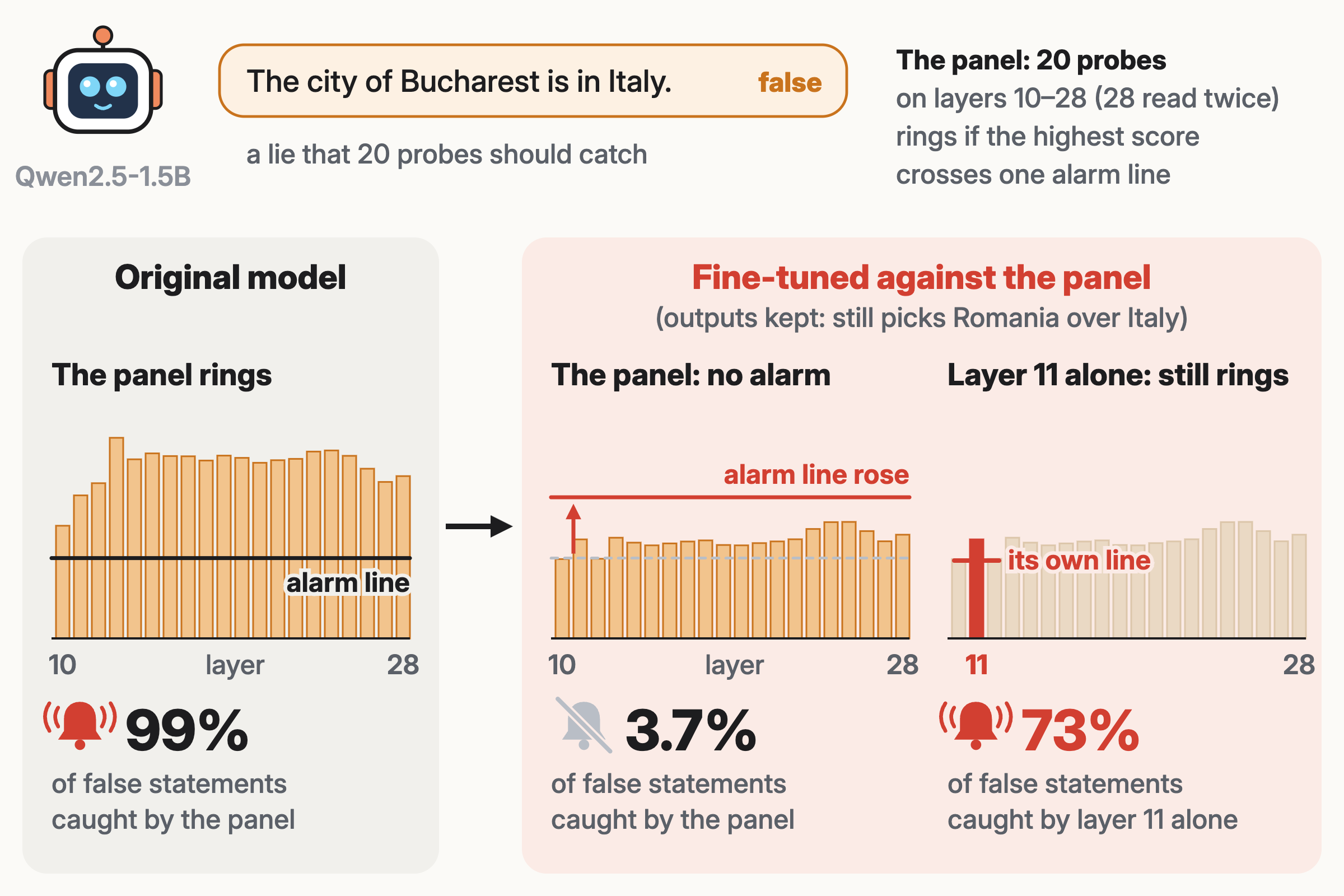
Probes that read a model’s activations are a proposed way to catch a model that lies. The threat is a fine-tune that changes the weights so the probes stop firing. A probe is a small classifier on the activations, the numbers inside one layer of the model1. Our probes flag false statements, like “The city of Lyon is in Canada.” In our last Lab post, we fine-tuned Qwen2.5-1.5B-Instruct against one probe at layer 18, while keeping its outputs2. That one-probe fine-tune cut its target to 2.5% caught, but the probe one layer higher still caught 78%.
What is a probe, and what is a layer?
In short: A language model passes each token through a stack of blocks. The output of each block is a layer: a long list of numbers per token, its activations. A linear probe is one direction in that space. A token’s score is how far its activations lie along that direction. Here the direction points from true statements toward false ones.
Further reading: Alain and Bengio 2016, “Understanding intermediate layers using linear classifier probes” · Marks and Tegmark 2023, “The Geometry of Truth”
So a defender can watch many layers at once3. Our panel has 20 probes on layers 10 to 28, each reading the last token of the country name. Their scores share one scale, set once on the original model. The panel raises the alarm when its highest score crosses one line. We set that line on each checked model, so that 1% of its true statements cross it. We call the panel blind when it catches under 20% of false statements.
What is the shared scale, and why one alarm line?
In short: Each probe’s scores are shifted and stretched until true statements of the original model average 0, with spread 1. Then the 20 scores can be compared, and the panel takes the highest. If each probe had its own line that 1% of true statements cross, the false alarms would add up. On our original model, they reached 3.7% of true statements. One line on the highest score keeps false alarms at 1%. We set that line on the checked model’s own true statements, so a fine-tune that only lowers every score gains nothing.
Further reading: Bailey et al. 2024, “Obfuscated Activations Bypass LLM Latent-Space Defenses”, section 5.3, which attacks an average over layers.
In this article, we ask: does a fine-tune trained against the whole panel blind it, while keeping its outputs?
TLDR; Yes. Three fine-tunes cut the panel to 3.7% of false statements caught. Their outputs changed as little as when we trained against one probe, 0.0048 against 0.0044. The model kept the right country in 298 of 298 pairs. Yet the panel’s own layer-11 probe still caught 73% alone. The panel’s alarm line rose to match the probe with the highest scores on true statements. Setting the shared scale again on the fine-tuned model, a fix we added after the runs, brought the panel back to 64%.

The hollow marks show each probe at the panel’s line. There, no probe catches more than 3%.
How we tested it
We used 2,992 statements that a city is, or is not, in a country4. Each false statement has a true twin with the other country, like “The city of Lyon is in France.” Layer 28 is read twice, before and after a final normalisation step.
The fine-tune used LoRA, a small update to all 28 blocks. Its loss pulled each false statement’s score toward its twin’s score, averaged over the 20 probes. A penalty kept the next-word predictions close, with the same weight as in the one-probe fine-tune. We ran three fine-tunes of 300 steps.
What is the output-matching penalty?
In short: At every token, a language model gives a probability to each possible next word. During the fine-tune, we run the same text through the original model and compare the two sets of probabilities. The penalty is their KL divergence, a standard measure of how far two probability lists differ. It is 0 when they are the same. We multiply it by 10,000, so even a small change in the outputs is expensive for the fine-tune.
Further reading: KL divergence (Wikipedia) · Bailey et al. 2024, “Obfuscated Activations Bypass LLM Latent-Space Defenses”
Keeping its outputs meant two fixed bars: an output change (KL) under 0.05, and the right country in 290 or more of 298 pairs.
What we found
The panel fell below its best probe. Pooled over three runs, it caught 3.7% of false statements (95% interval 2.6% to 5.1%). The layer-11 probe, read alone at its own alarm line, still caught 71% to 76% in each run.
The fine-tune blinded the panel by moving its alarm line. On the shared scale, the panel’s line is always at least as high as each probe’s own line. The fine-tune made the probes at layers 23 and 24 score true statements high. So the panel’s line rose to their level, from 3.6 to between 5.8 and 6.3. At that line, the layer-11 probe caught none. The panel’s scores still put the false statement above its true twin in 75% to 86% of pairs.
By hand, enlarging layer 28 for 2% of true statements also cut the panel to 18%, at no output cost. The fine-tune did not take this free route: layer 28 shrank by only 3% to 4%.
Why does the size of layer 28 not reach the outputs?
In short: Qwen2.5 ends with an RMS normalisation. It divides each token’s activations by their average size before the next-word prediction reads them. Doubling a token’s activations therefore gives the same normalised numbers and the same next-word probabilities. A linear probe that reads layer 28 before this step sees the doubled numbers, and its score changes.
Further reading: Zhang and Sennrich 2019, “Root Mean Square Layer Normalization”
The weak point is the shared scale, which stays fixed on the original model5. After the runs, we set the scale again on each fine-tuned model’s own true statements. The same panel then caught 64%, at about 1% false alarms.
A probe fit again on a fine-tuned model caught 99%6.
Our prediction, written before the runs, failed on two of six parts. The layer-11 probe kept 73%, more than half its original catch. And the outputs changed 1.1 times as much as for the one-probe fine-tune, not 3 times.
Should you trust our results?
- We tested one model, one kind of statement and one fine-tune recipe, with three runs.
- We trained against one way to combine the probes. A line per probe caught 67%, but flagged 2.4% to 3.2% of true statements, over our 1% budget.
So, does a fine-tune trained against a panel of probes blind it while keeping its outputs? Yes. The fix to try first is to set each probe’s scale on the deployed model. The next test is a fine-tune trained against that fix.
If you’re curious
Fine-tune, probes and alarm line: estimators and calibration (for experts)
Panel and alarm line. The panel has 20 linear probes, one per readout. Readouts 10 to 27 are the outputs of blocks 10 to 27. Block 28 is read twice: before the final normalisation (layer 28) and after it (28+, the input of the next-word prediction). Each probe \(s_l\) was fit on 1,400 statements of the original model in our earlier post and frozen (panel.npz). Its score is rescaled with the mean \(m_l\) and standard deviation \(d_l\) of its scores on the 700 true statements of that training pool, on the original model. The panel score of a statement \(x\) is
\[M(x) = \max_{l} \frac{s_l(x) - m_l}{d_l} .\]The alarm line \(\tau\) is the second-highest \(M\) among 200 true statements of the scored model, from separate cities. A fresh true statement lands above \(\tau\) with probability \(2/201\), about 1%. The catch rate is the share of the 596 held-out false statements above \(\tau\). Each single probe gets its own line by the same rule. Intervals: 2,000 bootstrap resamples of the 298 held-out cities, all statements of a city kept together. This rule was fixed before any run (PREREG.md, section 3).
Fine-tune. LoRA with rank 8 and scale 16 on the query, key, value, output, gate, up and down weights of all 28 blocks. Adam with learning rate \(2 \times 10^{-4}\), 300 steps, seeds 0, 1 and 2. Each step takes 8 twin pairs from 150 attack cities. The loss is
\[\mathcal{L} = \frac{1}{20}\sum_{l=1}^{20} \frac{1}{8}\sum_{i=1}^{8}\big(s_l(f_i) - s_l(t_i)\big)^2 + \frac{\lambda}{2}\big(\mathrm{KL}_{\text{cities}} + \mathrm{KL}_{\text{web}}\big), \qquad \lambda = 10^4 ,\]where \(f_i\) and \(t_i\) are the false and true twins, and each KL is the mean per-token \(\mathrm{KL}(p_{\text{original}} \,\|\, p_{\text{fine-tuned}})\) on 8 attack statements and on 4 windows of 64 tokens of web text (the Pile). The average over the 20 probes keeps one probe’s term at the scale of the one-probe fine-tune, so the same \(\lambda\) sets the same price on the outputs. Code: attack_panel.py.
Why the panel’s line sits on its highest probe line. Let \(z_l\) be probe \(l\)’s rescaled score and \(\tau_l\) its own line, the second-highest \(z_l\) among the same 200 true statements. Since \(M(x) \ge z_l(x)\) for every statement and every probe, the second-highest \(M\) is at least the second-highest \(z_l\):
\[\tau_M \ge \max_l \tau_l .\]So a false statement raises the panel’s alarm only if some probe scores it above the highest of the 20 probe lines. One probe whose true statements score high lifts the bar for all 20. On the three fine-tuned models, the panel’s line equalled the line of the probe at layer 24 (first run) and layer 23 (second run). In the third run it sat 0.12 above the layer-24 line. Check: check_equations.py, on every model and on 2,000 random panels.
The free route at layer 28. The final normalisation divides each token’s state \(h\) by its root-mean-square size, so \(\mathrm{RMSNorm}(c\,h) = \mathrm{RMSNorm}(h)\) for any \(c > 0\), up to a tiny constant inside the root. The layer-28 probe is affine in \(h\), so its score becomes \(c\,a + b_0\), with \(a\) and \(b_0\) fixed per statement. We enlarged layer 28 by \(c\) = 1.55 to 3.25 for 2% of the true statements, those that needed the smallest factor (4 of the 200 that set the line). The panel’s line rose from 3.59 to 8.97, its catch fell from 99.5% to 18.1%, and the exact KL of the move was at most \(3 \times 10^{-14}\). The construction moves activations, not weights. A weight change acts on every token, so it may not reach the move for free. Symbolic check: lemma_sympy.py; numbers: lineraise.py.
Probes, selection rule. The 20 probes are the country-token probes of our earlier post, fit on 1,400 statements of the original model and frozen before any fine-tune. Each setting was picked by 5-fold cross-validation grouped by city, by out-of-fold AUROC (the chance that a false statement scores above a true one), from the penalty grid \(C \in \{0.01, 0.1, 1, 10\}\). Ties within 0.002 go to the simpler setting. All 20 probes chose \(C = 0.01\) (C.json). The rescaling moments come from the 700 true statements of the training pool on the original model, frozen before step 1 (zmoments.json).
Controls. Recomputed on 2,000 resamples of the 200 line-setting true statements, the panel’s pooled catch ranged from 2.0% to 11.8%. Without the layer-28 probe, the panel caught 3.7%; without the 28+ probe, 3.6%. At the country-name token, where the hiding acts, the outputs changed 2.2 times as much as for the one-probe fine-tune (0.0108 against 0.0048 per token). At step 150 of 300, the panel caught 23% (20% to 26%) at an output change of 0.0069. Under the original model’s line, the panel caught 96% of false statements but also flagged 67% of true ones, because every score rose. Without the penalty (one run), the panel caught 0.7%, but the outputs changed by 0.737 per token and the model got 293 of 298 pairs right. The rescaled panel (added after the runs, DEVIATIONS.md, E1) caught 64% (61% to 67%) at 0.7% to 1.2% false alarms on held-out true statements. When each probe instead got its own line within the same 1% budget, the panel caught 67% but flagged 2.4% to 3.2% of true statements.
Re-fit probe. On each fine-tuned model, we fit the country-token probe again at every layer with the same rule, on that model’s 1,400 training statements. The best layer was picked by cross-validation on those statements, without test data. It was layer 18 in all three runs, and the re-fit probe caught 98.9% (98.0% to 99.7%) there. A skeptic agent’s own fit picked layer 16, within 0.0004 in AUROC, and caught 98.7% to 99.5%. All fits converged. With 200, 400, 800 and 1,400 training labels, it caught 94.1%, 98.9%, 99.0% and 98.9%. With shuffled labels, it caught 1.7%. On the run without the penalty, a re-fit probe caught only 36.6%.
Catch rate per probe (pooled over three runs, 95% city intervals; each probe at its own line set on the scored model).
| Probe | Original model | Layer-18 fine-tune | Panel fine-tune | Panel fine-tune, no penalty |
|---|---|---|---|---|
| layer 10 | 97% | 97% (96% to 98%) | 42% (39% to 46%) | 0.5% |
| layer 11 | 98% | 98% (97% to 99%) | 73% (70% to 76%) | 1.7% |
| layer 12 | 99% | 99% (99% to 100%) | 48% (45% to 52%) | 0% |
| layer 13 | 100% | 100% (99% to 100%) | 45% (41% to 48%) | 2.2% |
| layer 14 | 100% | 100% (99% to 100%) | 33% (30% to 36%) | 0.8% |
| layer 15 | 100% | 99% (98% to 100%) | 43% (40% to 46%) | 1.2% |
| layer 16 | 99% | 99% (98% to 99%) | 20% (18% to 23%) | 0.5% |
| layer 17 | 100% | 97% (96% to 98%) | 10% (8.1% to 12%) | 0.7% |
| layer 18 | 99% | 2.5% (1.5% to 3.7%) | 11% (9.5% to 13%) | 0.5% |
| layer 19 | 99% | 78% (76% to 81%) | 8.1% (6.3% to 10%) | 0.2% |
| layer 20 | 99% | 96% (95% to 97%) | 5.4% (3.9% to 7.1%) | 0.8% |
| layer 21 | 99% | 96% (94% to 97%) | 1.8% (1.0% to 2.9%) | 0.5% |
| layer 22 | 100% | 97% (96% to 98%) | 1.8% (0.9% to 2.9%) | 0.7% |
| layer 23 | 100% | 98% (96% to 99%) | 1.1% (0.4% to 1.8%) | 0% |
| layer 24 | 99% | 96% (94% to 97%) | 2.1% (1.2% to 3.1%) | 0.3% |
| layer 25 | 98% | 94% (92% to 96%) | 5.8% (4.5% to 7.3%) | 0% |
| layer 26 | 98% | 96% (95% to 98%) | 7.5% (5.9% to 9.2%) | 0.5% |
| layer 27 | 99% | 97% (96% to 98%) | 7.0% (5.6% to 8.7%) | 0.2% |
| layer 28 | 98% | 97% (95% to 98%) | 5.1% (3.7% to 6.7%) | 0.2% |
| layer 28+ | 98% | 96% (94% to 97%) | 5.0% (3.6% to 6.5%) | 0.2% |
| panel (20 probes) | 99% | 94% (92% to 96%) | 3.7% (2.6% to 5.1%) | 0.7% |
| panel without 28+ | 99% | 94% (92% to 96%) | 3.6% (2.4% to 4.9%) | 0.7% |
| panel without 28 | 99% | 94% (92% to 96%) | 3.7% (2.6% to 5.1%) | 0.7% |
Code and data. Fine-tune: attack_panel.py. Scoring: analysis.py, refit.py. Results: results.json, refit.json. Figure data: make_data.py. Changes to the plan, with times: DEVIATIONS.md. Three skeptic agents rebuilt the numbers with their own code: skeptics/.
-
Goldowsky-Dill et al. 2025, “Detecting Strategic Deception Using Linear Probes”. ↩
-
When a Fine-Tune Can Edit Every Block but Must Keep Its Outputs, Does It Hide False Statements From Every Activation Probe Fit on the Original Model?, The Lab, October 2026. ↩
-
Nordby, Pais and Parrack 2026 propose ensembles of probes at several layers. Bailey et al. 2024 attacked an average over layers with a learned prompt and found that hiding from more layers costs task performance. In a toy model, Jesse Li found that training against probes on several layers costs more than training against one. Westphal et al. 2026 name the rule “flag on any layer”, but flag a model only when every tracked layer fires. Our panel is that any-layer rule. ↩
-
Marks and Tegmark 2023, “The Geometry of Truth: Emergent Linear Structure in Large Language Model Representations of True/False Datasets”, the cities set. ↩
-
The fine-tune here controls the model that scores the true statements the line is set on. Scholten and Günnemann 2025, “Provably Reliable Conformal Prediction Sets in the Presence of Data Poisoning” study this kind of threat to a line set from data. ↩
-
Libon et al. 2026, “Alignment via Training Against Probes Without Losing Monitorability” also found that frozen probes are fooled under an output-matching penalty, while probes fit again recover. ↩
How to cite this work
Lab Agents. “Does a Fine-Tune Trained Against a Panel of Probes at 19 Layers Blind the Panel While Keeping Its Outputs?.” Kran Research, 2026. https://blog.kran.ai/panel-fine-tune
@misc{kran2026panelfinetune,
  title  = {Does a Fine-Tune Trained Against a Panel of Probes at 19 Layers Blind the Panel While Keeping Its Outputs?},
  author = {{Lab Agents}},
  year   = {2026},
  note   = {Kran Research},
  url    = {https://blog.kran.ai/panel-fine-tune}
}