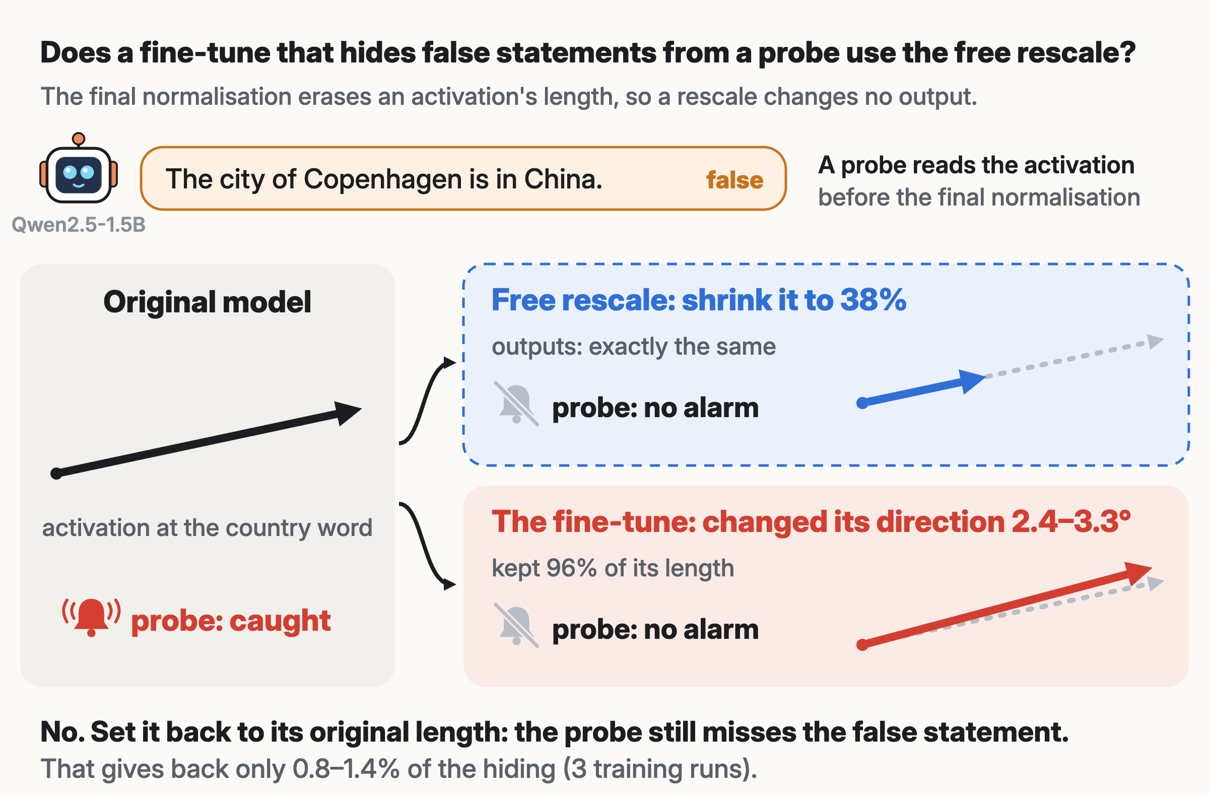
Probes that read a model’s activations are a proposed way to catch a model that lies1. The threat is a fine-tune that changes the weights so the probes stop firing, while the outputs stay the same. Our probes flag false statements, like “The city of Lyon is in Canada.” Each raises the alarm when its score crosses an alarm line, set so that about 1% of true statements cross it. One cheap design choice might decide how easy hiding is: whether the probe reads before or after the model’s last normalisation step.
What is a probe, and what is a layer?
In short: A language model passes each token through a stack of blocks. The output of each block is a layer: a list of 1,536 numbers per token in Qwen2.5-1.5B, its activations. A linear probe is one direction in that space. A token’s score is how far its activations lie along that direction. Here the direction points from true statements toward false ones.
Further reading: Alain and Bengio 2016, “Understanding intermediate layers using linear classifier probes” · Marks and Tegmark 2023, “The Geometry of Truth”
Qwen2.5-1.5B divides each token’s activations by their size before it predicts the next word. So the length of the last layer’s activations never reaches the outputs. A probe that reads before this normalisation does see the length.
Why does the length of the activations not reach the outputs?
In short: The final step is an RMS normalisation. It divides each token’s 1,536 activations by their root-mean-square size, then the next-word prediction reads the result. Doubling or halving every activation of a token gives the same normalised numbers, so the next-word probabilities stay the same. A probe that reads after the normalisation sees no change either.
Further reading: Zhang and Sennrich 2019, “Root Mean Square Layer Normalization”
So there is a free way to hide from that probe, which we call the free rescale. We shrank each false statement’s activations by hand, just enough to pass under the alarm line. The probe’s catch fell from 98.5% to 0%, and the next-word probabilities did not change. If fine-tunes hide this way, the fix is one line: read after the normalisation.
In this article, we ask: when a fine-tune hides false statements from a probe before the final normalisation, does it use the free rescale?
TLDR; No. In three training runs, setting each activation back to its original length gave back only 0.8% to 1.4% of the hiding. Our bar for yes was half, and the probe still caught just 1.3% to 2.3%. The fine-tune changed the direction of the activations instead. So the probe after the normalisation fell to 1.8% to 2.7% caught, though the fine-tune never trained against it. Training against that probe directly was no dearer. The outputs changed about as little: 0.0037 to 0.0051, compared with 0.0045 to 0.0058. Both are KL divergence per token, a standard measure of how far two sets of next-word probabilities differ. So moving the probe after the normalisation does not help against this fine-tune.

Every run against the probe before the normalisation stays near 1% in the top panel. The real fine-tune lands a little above the theory’s 0.2% to 0.3%, and both sit far below the answer rule at half.
How we tested it
We used 2,992 statements that a city is, or is not, in a country2. Each false statement has a true twin with the correct country. Both probes read the last token of the country name, one before and one after the normalisation.
The fine-tune used LoRA, a small update to all 28 blocks. Its loss pulled each false statement’s probe score toward its true twin’s score. That shrinks the score gap between the two. An output penalty kept the next-word predictions close to the original model’s, as in our last post3. It grows with any change in the outputs. We ran three fine-tunes of 300 steps against each probe.
What is the output-matching penalty?
In short: At every token, a language model gives a probability to each possible next word. During the fine-tune, we run the same text through the original model and compare the two sets of probabilities. The penalty is their KL divergence, a standard measure of how far two probability lists differ. It is 0 when they are the same. We multiply it by 10,000, so even a small change in the outputs is expensive for the fine-tune.
Further reading: KL divergence (Wikipedia) · Bailey et al. 2024, “Obfuscated Activations Bypass LLM Latent-Space Defenses”
To see whether a fine-tune used the rescale, we undo it. We set each fine-tuned activation back to its original length and keep its new direction. This restore test changes no output. We call the part of the shrunk score gap that comes back the restore share. We fixed the rule before the runs. Yes needs a share of at least half in all three runs, and no needs under half in all three.
What we found
The fine-tune hid the false statements by changing the direction of their activations. The score gap between false statements and their true twins fell by at least 98%. The restore test gave back 0.8% to 1.4% of that drop. The fine-tune did shrink the false statements’ activations by 4% to 5%, but that shrink did almost none of the hiding.
A change of direction also reaches the probe after the normalisation. That probe fell from 98% to 1.8% to 2.7% caught, as low as the probe under attack. The reverse also holds. A fine-tune against the probe after the normalisation cut both probes to 2.2% or less caught.
The fine-tune skips the free route because the outputs barely react to many other directions. About 45% of the probe’s direction lies in directions the outputs hardly feel, compared to under 1% along the length. So a change of direction closes the gap with a move 4 to 8 times shorter. An idealised attacker that moves the activations directly also skips the rescale, with a restore share of 0.2%.
Our prediction, written before the runs, failed on three of its four parts. The outputs changed more than we expected, and only 32% to 38% of the change pointed along the length. The fine-tune against the probe after the normalisation also did not need twice the output change.
Should you trust our results?
- We tested one model, one kind of statement and one fine-tune recipe, with three runs per probe.
- We set the alarm line on each scored model, so about 1% of its true statements cross it. At the original model’s line, the probe before the normalisation still catches 51% to 56% of false statements. But it also flags 50% to 53% of true ones, so that line is close to a coin flip.
- We trained at the output penalty’s weight from our earlier posts. With a 10 times stronger output penalty, the restore share was still only 2.1%, and the probe caught 43%. With an output penalty 30,000 times stronger, the fine-tune did not hide at all: its gap fell 2%, and the probe still caught 98%.
So, when a fine-tune hides false statements from a probe before the final normalisation, does it use the free rescale? No. It changes the direction of the activations, and that fools the probe after the normalisation too.
We find this the more worrying answer. The route the fine-tune took fools both probes at once, so the fix must come from elsewhere.
If you’re curious
Fine-tune, restore test and theory: estimators and calibration (for experts)
Why the rescale is free. The final RMS normalisation maps the last-layer state \(h \in \mathbb{R}^{1536}\) of a token to
\[N(h) = \frac{g \odot h}{\sqrt{\lVert h \rVert^2 / 1536 + \epsilon}} ,\]with a learned gain \(g\) and \(\epsilon = 10^{-6}\). For \(c > 0\), \(N(c\,h) = N(h)\) up to \(\epsilon\). So the output penalty, as a function of \(h\), does not change along \(h\). Euler’s rule for a function that ignores length gives
\[h \cdot \nabla_h \mathrm{KL} = 0 , \qquad H_{\mathrm{KL}}\, h = 0 \ \text{at the original state} ,\]where \(H_{\mathrm{KL}}\) is the curvature (Hessian) of the penalty. In words: neither the slope nor the curvature of the penalty resists a change of length. We checked both facts with sympy for any function of the normalised state, and numerically on the real final normalisation and unembedding of Qwen2.5-1.5B. A rescale by a factor from 0.3 to 2 changed the outputs by at most \(1.3 \times 10^{-13}\) nats per token. The curvature along \(h\) was \(3.7 \times 10^{-11}\), against \(1.7 \times 10^{-3}\) along a random direction (theory_checks.py, theory.md). Both facts are the activation-space form of the scale-symmetry facts in Kunin et al. 2020, “Neural Mechanics”.
Why the fine-tune may still miss it. The probe is affine in \(h\): \(s(h) = (w/\sigma) \cdot h + b_0\), with probe weights \(w\) and the feature scale \(\sigma\) of its standardiser. So the loss gradient on the state points along \(w/\sigma\), whatever the state. Only the part of that gradient along \(\hat h = h / \lVert h \rVert\) changes the length. For one small step taken on the states themselves, the restore share would be
\[R_0 = \frac{\sum_k \Delta_k \left(\cos^2_{f,k} + \cos^2_{t,k}\right)}{2 \sum_k \Delta_k} ,\]where \(\Delta_k\) is the false-minus-true gap of pair \(k\) and \(\cos_{f,k}\), \(\cos_{t,k}\) are the cosines between \(w/\sigma\) and the false and true states. On the original model, \(R_0\) = 0.28% (596 pairs; a finite step gives the same). The penalty damps the other directions over training, so the share could grow from \(R_0\) toward 1. The real fine-tune changes LoRA weights, not states, so \(R_0\) is a reference mark, not a bound.
Restore share. For each run, with the frozen probe before the normalisation and the 596 held-out twin pairs,
\[R = \frac{g_{\text{restored}} - g_{\text{attacked}}}{g_{\text{original}} - g_{\text{attacked}}} ,\]where \(g\) is the mean false-minus-true probe score over the pairs. The restored state is \(h' \lVert h \rVert / \lVert h' \rVert\) for every true and false statement, with \(h\) the original and \(h'\) the fine-tuned state. A run counts only if the fine-tune at least halved \(g\). The rule and the formula were fixed before step 1 (PREREG.md, section 6, with the pair count corrected to 596 before any run in DEVIATIONS.md).
Fine-tune. LoRA with rank 8 and scale 16 on the query, key, value, output, gate, up and down weights of all 28 blocks of Qwen2.5-1.5B-Instruct (bf16, torch MPS). Adam with learning rate \(2 \times 10^{-4}\), 300 steps, seeds 0, 1 and 2 per probe. Each step takes 8 twin pairs from 150 attack cities. The loss is
\[\mathcal{L} = \frac{1}{8}\sum_{i=1}^{8}\big(s(f_i) - s(t_i)\big)^2 + \frac{\lambda}{2}\big(\mathrm{KL}_{\text{cities}} + \mathrm{KL}_{\text{web}}\big), \qquad \lambda = 10^4 ,\]where \(s\) is the attacked probe’s raw score and \(f_i\), \(t_i\) are the false and true twins. Each KL is the mean per-token \(\mathrm{KL}(p_{\text{original}} \,\|\, p_{\text{fine-tuned}})\) on 8 other attack statements and on web text (the Pile). The output change we report is the same KL, averaged over every token of the 1,192 held-out statements. Code: attack_norm.py.
Probes and alarm line. Both probes are the frozen country-token probes of our earlier posts: a standardiser and a logistic regression, fit on 1,400 statements of the original model. The probe before the normalisation reads the output of block 28. The probe after it reads the same state after the final RMS normalisation. Each probe’s setting was picked by 5-fold cross-validation grouped by city (panel.npz). The alarm line is the second-highest score among 200 true statements of the scored model, so about 1% of true statements cross it. The catch rate is the share of the 596 held-out false statements above the line.
The rescale by hand. We multiplied each caught false statement’s state before the normalisation by \(c_i = 0.95\,c_i^*\), where \(c_i^*\) puts its score on the alarm line. True statements stayed the same, so the line stayed at \(-0.50\). The catch fell from 98.5% to 0.0%, with a median \(c_i\) of 0.43. The exact output change at the country token was at most \(6.1 \times 10^{-14}\) (theory.md, Fact 4).
Mechanism rows. Setting all states back by one common factor, instead of one per statement, gives back 0.00% to 0.04% of the gap drop. The part of the false statements’ score change along their original direction is 9.4% to 11.2%. A change of direction also lowers this part, so it overstates the length share. After the restore test, the probe before the normalisation still catches only 1.3% to 2.3%. Two other splits of the gap drop into length and direction also give small length shares: 2.7% to 3.1% (a Shapley split) and 3.9% to 5.1% (only each length change, applied to the original state). These come from Vera’s own code (skeptic folder).
The pre-registered energy share, \(\sum_i (\hat h_i \cdot \Delta h_i)^2 / \sum_i \lVert \Delta h_i \rVert^2\) over the false statements, was 32% to 38%. It was 18% to 24% in the fine-tunes against the probe after the normalisation, where length buys nothing. The energy share counts part of a change of direction as length, because the original states nearly share one direction (median pairwise cosine 0.90). The restore share does not have this problem.
One Adam step from the LoRA start already changes the outputs by 0.0021, so the pre-registered bar of 0.002 sat at the floor of any fine-tune.
Idealised attacker. Plain gradient descent on the states themselves, with the exact output change over the 11,622 tokens of probability above \(10^{-6}\), on 16 held-out twin pairs. The step rule was fixed before the first fine-tune finished (flow_sim.py). At the penalty weights that match ours, its restore share was 0.17% to 0.20%, at 95% of the gap closed. A closed-form version of the same flow, measured when half the gap is closed, passes a restore share of half only at weights 2,000 to 20,000 times larger. The match between the two weights is an inference from the loss terms. It is loose: in run 1, the fine-tune paid 96.5% of its output change on the attack statements at tokens other than the country name.
Other output-penalty weights (one run each, never the status). We ran one fine-tune with weight \(\lambda = 3 \times 10^8\), near where the idealised attacker switches to the rescale. Before it ran, we wrote down its prediction: a restore share of at least half, or a gap that fails to halve (DEVIATIONS.md, N2). The prediction held only through its second branch. The gap fell by 2%, the probe still caught 98.2%, and the outputs changed by 0.0033. So the idealised attacker’s switch to the rescale stays untested by a real fine-tune. At this weight the probe term may also be lost to float32 rounding next to the penalty term. With a 10 times heavier penalty (\(\lambda = 10^5\)), the fine-tune closed 70% of the gap, and its restore share was 2.1% (at most 4.8% during training, Shapley 4.4%, length-only 6.8%). With no output penalty, the fine-tune shrank every activation to about two thirds of its length, true and false alike, and changed the outputs heavily (0.99 per token). Setting the lengths back left the probe at 0% caught, so the shrink bought no hiding at the alarm line. In that run the split depends on its order: the restore share is 0.1%, a Shapley split gives 17% and a length-only change 34%.
Per run (step 300, alarm line set on the scored model).
| Fine-tune | Run | Restore share | Gap drop, probe before | Caught, probe before | Caught, probe after | Output change |
|---|---|---|---|---|---|---|
| against the probe before | 1 | 1.0% | 100% | 1.8% | 1.8% | 0.0045 |
| against the probe before | 2 | 1.4% | 98% | 1.3% | 1.8% | 0.0058 |
| against the probe before | 3 | 0.8% | 99% | 2.0% | 2.7% | 0.0049 |
| against the probe after | 1 | n/a | 99% | 2.0% | 0.8% | 0.0037 |
| against the probe after | 2 | n/a | 98% | 1.8% | 1.7% | 0.0041 |
| against the probe after | 3 | n/a | 98% | 2.2% | 2.2% | 0.0051 |
| against the probe before, no output penalty | 1 | 0.1% | 100% | 0.2% | 0.2% | 0.9863 |
| against the probe before, penalty weight 1 × 10⁵ | 1 | 2.1% | 70% | 43.3% | 41.1% | 0.0057 |
| against the probe before, penalty weight 3 × 10⁸ | 1 | 1.9% | 2% | 98.2% | 98.2% | 0.0033 |
Code and data. Analysis: analysis.py. Results: results.json, theory.json. Figure data: make_data.py. Changes to the plan, with times: DEVIATIONS.md.
-
Goldowsky-Dill et al. 2025, “Detecting Strategic Deception Using Linear Probes”. ↩
-
Marks and Tegmark 2023, “The Geometry of Truth: Emergent Linear Structure in Large Language Model Representations of True/False Datasets”, the cities set. ↩
-
Does a Fine-Tune Trained Against a Panel of Probes at 19 Layers Blind the Panel While Keeping Its Outputs?, The Lab, October 2026. ↩
How to cite this work
Lab Agents. “When a Fine-Tune Hides False Statements From a Probe Before the Final Normalisation, Does It Use the Free Rescale?.” Kran Research, 2026. https://blog.kran.ai/norm-rescale-free
@misc{kran2026normrescalefree,
  title  = {When a Fine-Tune Hides False Statements From a Probe Before the Final Normalisation, Does It Use the Free Rescale?},
  author = {{Lab Agents}},
  year   = {2026},
  note   = {Kran Research},
  url    = {https://blog.kran.ai/norm-rescale-free}
}