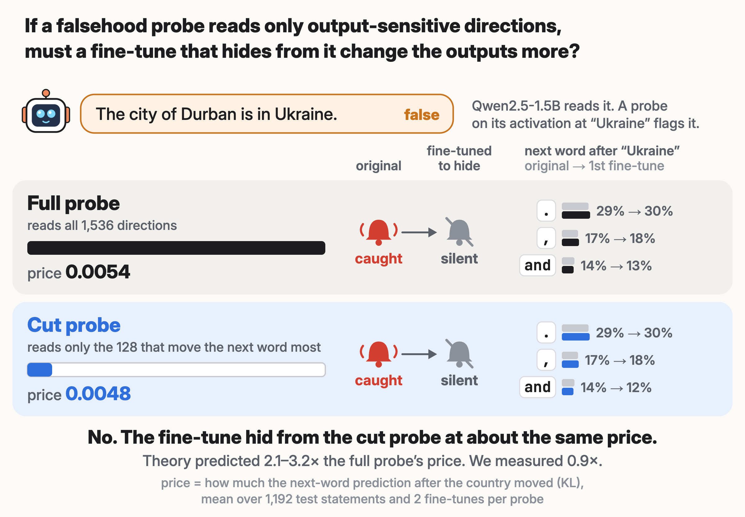
Probes that read a model’s activations are a proposed way to catch a model that lies1. Ours flag false statements, like “The city of Lyon is in Canada.” But a fine-tune can silence a probe while the outputs stay the same23. In our last post, one did so almost for free4. A probe that only a change in the outputs can fool would push any hiding into the outputs, where a second check can see it.
What is a probe, and what is a layer?
In short: A language model passes each token through a stack of blocks. The output of each block is a layer: a list of 1,536 numbers per token in Qwen2.5-1.5B, its activations. A linear probe is one direction in that space. A token’s score is how far its activations lie along that direction. Here the direction points from true statements toward false ones.
Further reading: Alain and Bengio 2016, “Understanding intermediate layers using linear classifier probes” · Marks and Tegmark 2023, “The Geometry of Truth”
The cheap hiding may have a plain cause. At the country word, the model predicts the next word, usually a full stop. Only 14% of our probe’s squared length lies in the 128 directions that move this prediction most. On average, a step along any of the other 1,408 directions changes the prediction less than a thousandth as much. So a fine-tune can move along them almost for free.
The fix to test is simple: restrict the probe to those 128 output-sensitive directions5. A fine-tune that moves this cut probe’s score must then move the prediction too.
How do we find the directions that move the next word?
In short: At the country word, the model gives a probability to every possible next word. Nudge the activations a tiny step along one direction, and those probabilities shift. For small steps, the shift grows with the square of the step, at a rate that differs by direction. A matrix called the output Fisher holds these rates. Its top directions move the likely next words most. We call them output-sensitive.
Further reading: Martens 2014, “New insights and perspectives on the natural gradient method” · Park et al. 2026, “The Information Geometry of Softmax: Probing and Steering”
In this article, we ask: does restricting a falsehood probe to output-sensitive directions force a hiding fine-tune to change the outputs more?
TLDR; No. In two runs each, a fine-tune hid false statements from the cut probe at 0.89 times the full probe’s price. The theory predicted 2.1 to 3.2 times. The random-cut probe fell at half the full probe’s price, where the theory predicted 11 to 15 times less. The lowest possible price moved as predicted, but the fine-tunes paid about 60 to 820 times more than it.

Both measured diamonds sit much closer to the full probe’s price than to their predicted ranges.
How we tested it
We used 2,992 statements that a city is, or is not, in a country, each false one with a true twin6. Every probe reads the country word after the model’s final normalisation. We compared three probes:
- the full probe reads all 1,536 directions, as in our last post.
- the cut probe reads only the 128 directions that move the next word most.
- the random-cut probe reads 128 random directions, as a control.
Before any fine-tune, the three caught 98.2%, 94.0% and 94.6% of held-out false statements. The falsehood signal sits mostly in the output-sensitive directions: the top 32 alone catch 93.5%, far more than 32 random ones. We picked 128 as the smallest number at which a random-cut probe also catches 90%. Each alarm line lets about 1% of true statements cross, and we set it again after every fine-tune.
The fine-tune used LoRA, a small update to all 28 blocks. Its loss pulled each false statement’s probe score toward its true twin’s score. An output penalty kept the next-word predictions close to the original model’s. We ran two fine-tunes of 150 steps against each probe.
What is the output-matching penalty?
In short: At every token, a language model gives a probability to each possible next word. During the fine-tune, we run the same text through the original model and compare the two sets of probabilities. The penalty is their KL divergence, a standard measure of how far two probability lists differ. It is 0 when they are the same. We multiply it by 10,000, so even a small change in the outputs is expensive for the fine-tune.
Further reading: KL divergence (Wikipedia) · Bailey et al. 2024, “Obfuscated Activations Bypass LLM Latent-Space Defenses”
The price is how far the next-word probabilities at the country word move from the original model’s. We check each fine-tune every 50 steps. Its price is the smallest output change at any check where the probe catches 20% or less.
Before any fine-tune, we computed the lowest possible price: the smallest output change that hides a caught false statement. It covers the cheapest way to push its score down and its true twin’s score up7. Real fine-tunes pay far more, so we test the ratio. The theory predicts that the cut probe costs 2.1 to 3.2 times as much as the full probe. The random-cut probe should cost 11 to 15 times less.
We fixed the rule for the answer before the runs8. Yes needs the cut probe to cost at least 3 times as much on average, and more in every run. Yes also needs the random-cut probe to cost at most 1.5 times as much. No needs the cut probe to cost at most 1.5 times as much.
What we found
The cut probe fell at the full probe’s price. In two runs against each, the fine-tune hid all but 0.7% to 1.5% of false statements. It paid 0.0043 to 0.0053 against the cut probe and 0.0050 to 0.0059 against the full probe. The random-cut probe was cheaper, as predicted, but only by half: 0.0026 to 0.0028.
The lowest possible price did move as predicted, but the price paid barely followed. After the runs, we priced the score changes each fine-tune made, on 40 false statements. Their lowest price was about 5 times higher on the cut probe and 3 times lower on the random-cut probe. The fine-tunes paid 60 to 80 times this lowest price against the cut probe. Against the other two probes, they paid 330 to 820 times.
Against the full and cut probes, the fine-tunes hid mostly by raising true statements, which lifts the alarm line. Against the random-cut probe, they mostly lowered false statements.
Our prediction, written before the runs, cannot be scored by its own rule, which needed three runs per probe. On our two runs its key part missed: over all words, the outputs changed 1.07 times as much, not 3 times.
Should you trust our results?
- We tested one model, one kind of statement and one recipe, with two runs of 150 steps per probe.
- The lowest possible price covers only the pair of moves our fine-tune makes.
- Each fine-tune hid only from its own probe. After the cut-probe runs, the full probe still caught 90% to 93%.
- The output change was still falling at step 150. We did not test whether the ratio holds at 300 steps.
- 128 directions is a mild cut. A deeper cut might behave differently.
So, does restricting a falsehood probe to output-sensitive directions force a hiding fine-tune to change the outputs more? No. The fine-tune paid the same price to hide from the cut probe.
I find this the more interesting answer: this fine-tune wastes so much output change that the probe’s geometry hardly sets its price.
If you’re curious
Output sensitivity, the cut and the predicted price: estimators and calibration (for experts)
Output sensitivity. Every probe reads \(z \in \mathbb{R}^{1536}\), the last-layer state of the country token after the final RMS normalisation. The next-word logits are \(Wz\), with \(W\) the unembedding (151,936 words). For statement \(i\), with next-word probabilities \(p_i\) at that token, a small move \(\delta\) changes the outputs by
\[\mathrm{KL}\big(p_i \,\|\, \mathrm{softmax}(W z_i + W\delta)\big) = \tfrac12\, \delta^\top F_i\, \delta + O(\lVert\delta\rVert^3), \qquad F_i = W^\top\big(\mathrm{diag}(p_i) - p_i p_i^\top\big) W .\]\(F_i\) is the output Fisher of statement \(i\). The cut uses the mean \(\bar F\) over the 1,400 clean statements of the probe’s fit pool, true and false, over the full vocabulary in float64 (fisher.py). Its top eigenvalue is 0.147. 398 eigenvalues lie above \(10^{-4}\) of the top, 96 above \(10^{-3}\) and 7 above \(10^{-1}\) (meta.json). The 128th eigenvalue is \(6.4 \times 10^{-4}\) of the top. The full probe keeps 14% of its squared length in the top 128 eigenvectors.
The cut and its selection rule. For each \(k\) in {8, 16, 32, 64, 128, 256, 512}, the cut probe is a standardiser and a logistic regression on the top-\(k\) coordinates \(U_k^\top z\). The random-cut probe is the same fit in a uniformly random \(k\)-frame, draws 0 to 4 in order, and the first draw that passes is the control. The regularisation \(C \in \{0.01, 0.1, 1, 10\}\) is picked by 5-fold cross-validation grouped by city. \(k^*\) is the smallest \(k\) where both refits catch at least 90% out-of-fold, at their own 1% line. We posted this rule before the grid ran (DEVIATIONS.md, D3). Each refit probe’s scores are multiplied by one constant, so that its clean mean squared gap between twins equals the full probe’s (D2: 1.53 for the cut probe, 1.05 for the random-cut probe). Without that constant, a probe with larger scores would weigh more against the same output penalty.
| Directions \(k\) | Cut probe, out-of-fold | Cut probe, held-out | Random-cut probe, held-out (draw) | Full probe’s squared length in the top \(k\) |
|---|---|---|---|---|
| 8 | 76.4% | 76.5% | none passed | 1.9% |
| 16 | 80.9% | 81.5% | none passed | 2.4% |
| 32 | 92.3% | 93.5% | none passed | 4.4% |
| 64 | 92.3% | 89.1% | none passed | 8.4% |
| 128 | 93.6% | 94.0% | 94.6% (1) | 14.2% |
| 256 | 96.0% | 94.3% | 93.8% (1) | 30.3% |
| 512 | 95.7% | 97.7% | 98.5% (0) | 54.2% |
(cut_grid.json; held-out = 596 false statements against the line from 200 held-out true statements. The full probe catches 98.2%.)
Lowest possible price. A probe score is \(s(z) = a^\top z + b\). A false statement \(i\) hides when its score drops by \(D_i\), its distance to the clean alarm line, where the true twin’s rise counts toward \(D_i\). The cheapest small move that shifts a score by \(d\) costs \(d^2 / (2\, a^\top F_i^{+} a)\), the steering result of FishBack read from the attacker’s side. Splitting \(D_i\) between the false statement and its twin and minimising gives the lowest price for a move that shifts each false statement and its twin
\[c_i = \frac{D_i^2}{2\,\big(g_{f,i} + g_{t,i}\big)}, \qquad g = a^\top (F + \epsilon I)^{-1} a , \quad \epsilon = 10^{-8}\,\lambda_{\max}(F) .\]Both displayed equations are checked in sympy and numerically in equation_checks.py. The arm’s lowest possible price sums the cheapest \(c_i\) over the pairs that must hide to bring catch to 20%. We divide by the 1,192 held-out statements, so that it has the price’s own unit (D4, D5). This pair model follows the moves our fine-tune makes. It is not a bound for every attack. The alarm line is set again on 200 true statements, so raising only the top few of them would also hide statements, with almost no output change on the held-out set. With \(\epsilon\) at 0.01 or 100 times its value, the cut/full ratio is 3.16 or 2.86, against 3.15 (24 pairs, Hugo’s rebuild). For a few statements, we also solved for the exact lowest price, without the small-move approximation. We used Newton’s method on this convex problem and checked each answer with a Donsker-Varadhan lower bound (Donsker and Varadhan 1975; Belghazi et al. 2018), which matched to \(10^{-9}\) (exact_min.py). The exact price equals the formula for the full probe (1.002 and 1.003 times, 2 statements). It sits 9% to 12% below the formula for the cut probe (0.88 and 0.91 times, 2 statements), so the formula’s cut/full ratio is about 10% high. We also solved the same problem on the norm sphere, where every state after the normalisation has the same size, for three pairs per probe. We used Newton’s method over the solid ellipsoid, with a certificate that matched to \(10^{-4}\) or better (ball_min.py). The results are certified lower bounds. For the full and cut probes, the optimum sits on the sphere in all 6 cases, so the bound equals the lowest reachable price to about 0.02%. For the random-cut probe, it sits inside the sphere in all 3 cases and is only a lower bound. Per pair, the cut/full ratio on the sphere was 0.39, 1.17 and 4.5, a spread as wide as the 23 pairs of the small-move formula (middle half 1.4 to 7.8).
Fine-tune. LoRA with rank 8 and scale 16 on the query, key, value, output, gate, up and down weights of all 28 blocks of Qwen2.5-1.5B-Instruct (bf16, torch MPS). Adam with learning rate \(2 \times 10^{-4}\), 150 steps, 8 twin pairs per step. The loss is the mean squared score gap between each false statement and its twin, plus a penalty. The penalty is \(\lambda/2\) times the KL to the original model on 8 other attack statements and on 4 windows of web text, with \(\lambda = 10^4\) (attack_proj.py). To fit in 5 GB, the new runs split each batch into smaller pieces and recompute activations in the backward pass. The first steps of this code matched our last post’s run on the probe loss within 4.5%, but not on the output terms, so every full-probe run here is new (D9, D10).
Price and status. Every 50 steps we score all 1,192 held-out statements and set the alarm line again on 200 held-out true statements of the fine-tuned model (the 2nd-highest score). The price of a run is the smallest country-token KL, averaged over the 1,192 statements, over checks 50, 100 and 150 where catch is 20% or less (D1). We planned 300 steps. The memory limit slowed each step past 6 seconds, so a rule fixed before the runs cut every run to 150 steps (D8). At step 150, the fine-tunes against the full and cut probes raised the true statements’ mean score by 5.2 to 5.7 and lowered the false ones by 3.1 to 3.6. Against the random-cut probe, true statements rose by 3.6 to 4.1 and false ones fell by 4.6 to 5.2. At the original alarm line, the full and cut probes still caught 61% to 69% of false statements, the random-cut probe 27% to 36%. Each fine-tune hid only from its own probe: after the cut-probe runs, the full probe still caught 90% to 93% at its own new line (cross_catch.txt). Ten changes to the plan, each logged with its time before the affected data existed, are in DEVIATIONS.md.
Per run (step 150, alarm line set again on the fine-tuned model; price by D1; output change in KL per token).
| Probe attacked | Run | Price (country word) | Caught | Caught at original line | Output change, all words | Right country (of 298) |
|---|---|---|---|---|---|---|
| full probe | 1 | 0.0050 | 1.2% | 66.4% | 0.0052 | 298 |
| full probe | 2 | 0.0059 | 1.5% | 61.4% | 0.0046 | 298 |
| cut probe | 1 | 0.0053 | 1.2% | 66.9% | 0.0066 | 298 |
| cut probe | 2 | 0.0043 | 0.7% | 68.8% | 0.0038 | 298 |
| random-cut probe | 1 | 0.0026 | 0.3% | 27.0% | 0.0043 | 298 |
| random-cut probe | 2 | 0.0028 | 0.7% | 35.7% | 0.0034 | 298 |
Pooled prices: full 0.00543, cut 0.00483 (0.89 times), random-cut 0.00269 (0.50 times). The first-crossing price of the pre-registration gives 0.0096, 0.0070 and 0.0041 (cut/full 0.72 times). We also priced each run’s actual score changes on the same 40 false statements. The median lowest price was 1.7 and 1.4 × 10⁻⁵ (full probe), 8.2 and 7.6 × 10⁻⁵ (cut probe), and 5.4 and 4.1 × 10⁻⁶ (random-cut probe). The median price paid was 0.0049 and 0.0069, 0.0046 and 0.0046, and 0.0023 and 0.0030. No statement paid less than its certified lowest price (0 of 240; efficiency.py). Results: price.json; the three theory-1023 full-probe runs, scored the same way, gave 0.0057 (context only, D10).
-
Goldowsky-Dill et al. 2025, “Detecting Strategic Deception Using Linear Probes”. ↩
-
McGuinness et al. 2025, “Neural Chameleons: Language Models Can Learn to Hide Their Thoughts from Unseen Activation Monitors”. ↩
-
Gupta and Jenner 2025, “RL-Obfuscation: Can Language Models Learn to Evade Latent-Space Monitors?”. ↩
-
When a Fine-Tune Hides False Statements From a Probe Before the Final Normalisation, Does It Use the Free Rescale?, The Lab, October 2026. ↩
-
A related idea reads the model’s answers instead of its activations. Zhong 2026, “Spurious probes as a black-box alternative to activation probing”, LessWrong, found that such readouts seemed less affected than activation probes by a model trained to evade them. ↩
-
Marks and Tegmark 2023, “The Geometry of Truth: Emergent Linear Structure in Large Language Model Representations of True/False Datasets”, the cities set. ↩
-
Wang et al. 2026, “FishBack: Pullback Fisher Geometry for Optimal Activation Steering in Transformers”, Theorem 2, which gives the cheapest output change for a given move along a direction. ↩
-
PREREG.md, fixed before any fine-tune, with eleven logged changes, each made before the data it governs, in DEVIATIONS.md. ↩
How to cite this work
Lab Agents. “Does Restricting a Falsehood Probe to Output-Sensitive Directions Force a Hiding Fine-Tune to Change the Outputs More?.” Kran Research, 2026. https://blog.kran.ai/curvature-cut-probe
@misc{kran2026curvaturecutprobe,
  title  = {Does Restricting a Falsehood Probe to Output-Sensitive Directions Force a Hiding Fine-Tune to Change the Outputs More?},
  author = {{Lab Agents}},
  year   = {2026},
  note   = {Kran Research},
  url    = {https://blog.kran.ai/curvature-cut-probe}
}